In-Class Assignment 8#
Exploring Heat Transfer via Convection with MESA#
Learning Objectives#
identify convective and radiative regions using MESA models and analytical expressions
explain convective behavior in advanced burning massive stars and Solar-like stars
import numpy as np
import matplotlib.pyplot as plt
import pandas as pd
a. Convection in Massive Stars#
Download the following model files locally. These data were produced using the MESA 20m_ms_convection_profile.data test suite.
New \(20.0 M_{\odot}\) Main-Sequence profile data: 20m_ms_convection_profile.data;
Plot the adiabatic gradient
grada, the radiative gradientgradr, and the Ledoux term (gradL) as a function of radius (in units of Rsun) using the MESA data.
Hint: You may want to set your ylim to
0.2,1
Locate the approximate fractional radius and annotate where the Schwarzchild Criterion $\( \nabla < \nabla_{\rm{ad}} \)$ is volated and fill in the convective region of the star using
plt.fill_betweenx().
Hint: You may want to set your yrange to
(0,1)
We found that the limiting cases for \(\nabla_{\rm{ad}}\) is: 0.4 for an ideal gas without radiation and 0.25 for a radiation-dominated gas. Label these two limits on the same plot using
plt.axhlineDescribe in a few sentences where is the model convective and way? Also, describe where \(\nabla_{\rm{ad}}\) is closer to one limit or the other and why? What does it mean when \(\nabla_{\rm{L}}=0\)?
Hint: Compare with Pols Fig. 5.4.
## load MESA data here
#massive_star_ms_profile = pd.read_csv('data/20m_ms_convection_profile.data',sep=r'\s+',header=4)
#list(massive_star_ms_profile)
rsun_cgs = 6.96e10 # cm
# example reading a variable from the profile data
#massive_star_ms_profile_gradrad = massive_star_ms_profile['###
#massive_star_ms_profile_radius_cm = massive_star_ms_profile['##
#massive_star_ms_profile_gradad = ##
#massive_star_ms_profile_gradL = ##
## 1-3 result here
#plt.title('20$M_\odot$ Main-Sequence MESA Model')

#plt.plot(##
#         ##,label=r'$\nabla_{\rm{ad}}$')


#plt.axhline(##,ls='--',lw=1,color='cyan') # ideal gas nabla ad
#plt.axhline(##,ls='--',lw=1,color='cyan') # radiation dominated gas nabla ad

#plt.fill_betweenx((0,1),#,##,color='dodgerblue',alpha=0.5) # fill in convective zone

#plt.axvline(##,color='k',ls='--',lw=1) # convective zone boundary

#plt.ylim(
#plt.xlim(

#plt.legend()
#plt.xlabel(r'$r/R_{\odot}$')
#plt.ylabel(r'$\nabla$')
4. result here#
Radiation dominated, lower \(\nabla_{\rm{ad}}\) in the atmosphere and it is in fact convective. When \(\nabla_{\rm{L}}=0\), the composition is uniform.
b. Convection in a Solar-Like Star#
Download the following model files locally. These data were produced using the MESA 1m_pre_ms_to_wd.data test suite.
\(1.0 M_{\odot}\) Main-Sequence profile data: 1m_pre_ms_to_wd.data;
Plot the adiabatic gradient
gradaand the radiative gradientgradras a function of radius (in units of Rsun) using the MESA data.Locate the approximate fractional radius and annotate where the Schwarzchild Criterion $\( \nabla < \nabla_{\rm{ad}} \)$ is volated and fill in the convective region of the star using
plt.fill_betweenx().
Hint: You may want to set your yrange to
(0,1)
We found that the limiting cases for \(\nabla_{\rm{ad}}\) is: 0.4 for an ideal gas without radiation and 0.25 for a radiation-dominated gas. Label these two limits on the same plot using
plt.axhlineDescribe in a few sentences where is the model convective and way? Also, describe where \(\nabla_{\rm{ad}}\) is closer to one limit or the other and why?
Hint: Compare with Pols Fig. 5.4.
## load b data here
#massive_star_ms_profile = pd.read_csv('data/1m_pre_ms_to_wd.data',sep=r'\s+',header=4)
#massive_star_ms_profile_gradrad = massive_star_ms_profile['##
#massive_star_ms_profile_radius_cm = massive_star_ms_profile['##
#massive_star_ms_profile_gradad = massive_star_ms_profile['##
# this data set doesnt have gradL :(
## 1-3 result here
#plt.plot(##,label=r'$\nabla_{\rm{ad}}$')

#plt.plot(##,label=r'$\nabla_{\rm{rad}}$')

#plt.title('1$M_\odot$ Main-Sequence MESA Model')

#plt.fill_betweenx(#

#plt.axvline(#

#plt.legend()
#plt.xlabel(r'$r/R_{\odot}$')
#plt.ylabel(r'$\nabla$')
c. Convection in an Advanced Massive Star#
Download the following model files locally. These data were produced using the MESA 15m_core_O_burning_profile.data test suite.
New \(15 M_{\odot}\) Core O-Burning profile data: 15m_core_O_burning_profile.data;
Plot the adiabatic gradient
gradaand the radiative gradientgradras a function of massmass(in units of Msun) using the MESA data from 0 to 7 Msun.On the same plot, plot the normalized nuclear energy generation rate
eps_nucand the non-normalized mean molecular weight. Set the ylim to 0,2.Locate the approximate fractional radius and annotate where the Schwarzchild Criterion $\( \nabla < \nabla_{\rm{ad}} \)$ is volated and fill in the convective region of the star using
plt.fill_betweenx().
Hint: There are at least two in this model.
Hint: You may want to set your yrange to
(0,2)
Describe in a few sentences where is the model convective and way? Also, describe where \(\nabla_{\rm{ad}}\) is closer to one limit or the other and why?
Hint: Compare with Farmer et al. 2016
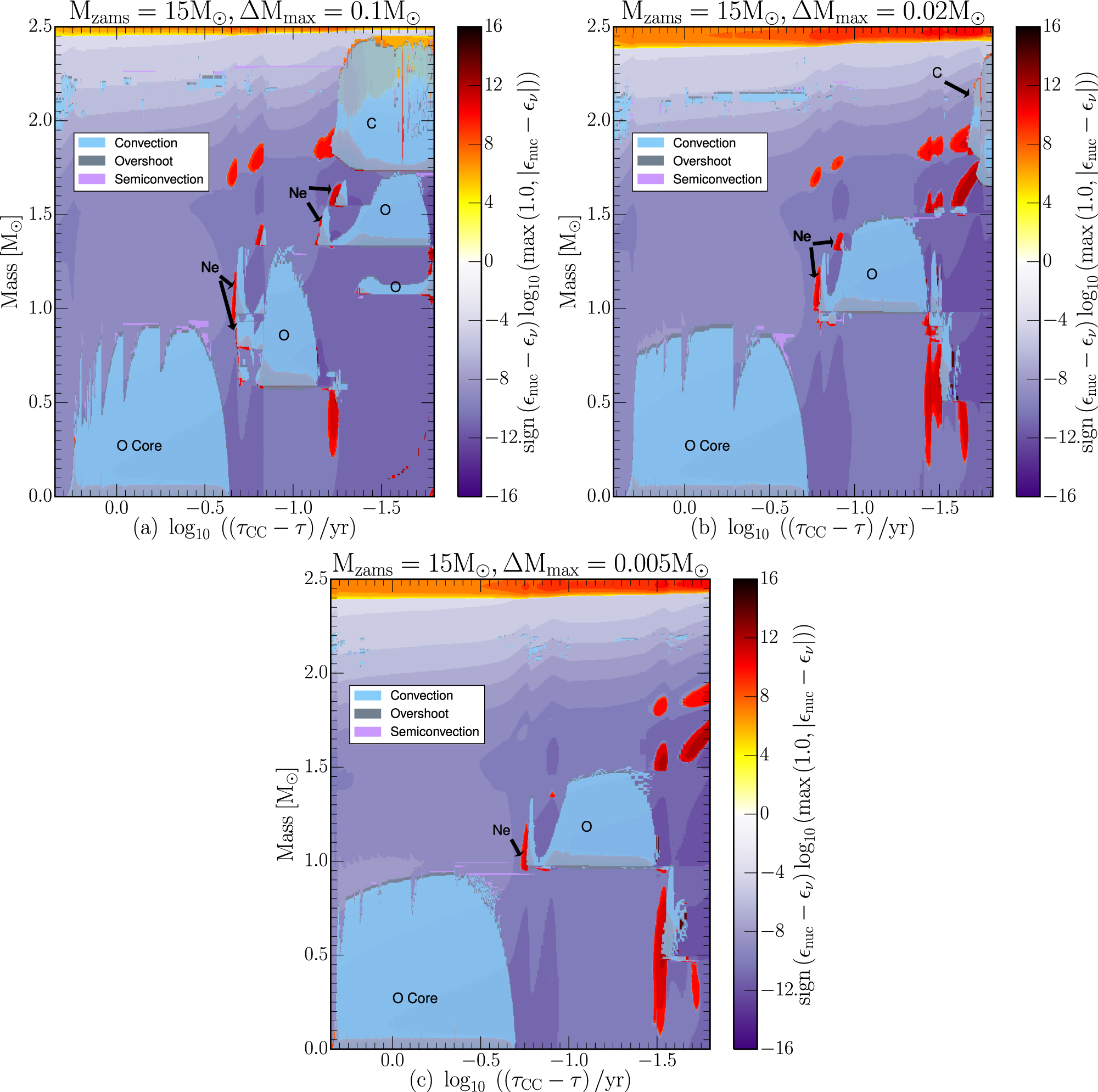
Stars might be like onions after all?? Not parfaits..
## load c data
#massive_star_ms_profile = pd.read_csv('data/15m_core_O_burning_profile.data',sep=r'\s+',header=4)
#massive_star_ms_profile_gradrad = massive_star_ms_profile['##
#massive_star_ms_profile_mass = massive_star_ms_profile['##
#massive_star_ms_profile_gradad = massive_star_ms_profile['##
#massive_star_ms_profile_eps_nuc = ##
#massive_star_ms_profile_mu = ##
# 1 - 3 result here
#plt.plot(##,label=r'$\nabla_{\rm{ad}}$')

#plt.plot(##,label=r'$\nabla_{\rm{rad}}$')

#plt.plot(##,label=r'$\epsilon_{\rm{nuc}}$') # dont forget to normalize by max

#plt.plot(##,label=r'$\mu$')

#plt.title('15$M_\odot$ Core O-Burning MESA Model')

#plt.legend()
#plt.xlabel(r'$m/M_{\odot}$')
#plt.ylabel(r'$\nabla,\mu,\epsilon_{\rm{nuc,normalized}}$')