In-Class Assignment 2

Credit: These exercises follow from work by Mike Zingale’s computational lectures.

We will be picking up from ICA1. These exercises require the solutions from ICA1 and are included here.

from sympy import init_session
init_session(use_latex="mathjax")
%matplotlib inline

IPython console for SymPy 1.13.3 (Python 3.11.8-64-bit) (ground types: python)

These commands were executed:
>>> from sympy import *
>>> x, y, z, t = symbols('x y z t')
>>> k, m, n = symbols('k m n', integer=True)
>>> f, g, h = symbols('f g h', cls=Function)
>>> init_printing()

Documentation can be found at https://docs.sympy.org/1.13.3/

1. stellar model

rho = symbols('rho', cls=Function)
rhoc = symbols('rho_c')
qc = symbols('q_c')
Pc = symbols('P_c')
G = symbols('G')
Mstar, Rstar = symbols('M_\star R_\star')
r = symbols('r')
xi = symbols('xi')
mu = symbols('mu')
k = symbols('k')
m_u = symbols('m_u')

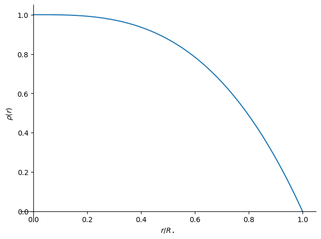
Imagine a star has a density profile of the form:

\[\rho(r) = \rho_c \left [ 1 - \left (\frac{r}{R_\star} \right )^3 \right ]\]

where \(\rho_c\) is the central density.

rho = rhoc * (1 - (r/Rstar)**3)
rho

\[\displaystyle \rho_{c} \left(1 - \frac{r^{3}}{R_{\star}^{3}}\right)\]

z = (rho/rhoc).subs(r, xi*Rstar)
plot(z, (xi, 0, 1), xlabel=r"$r/R_\star$", ylabel=r"$\rho(r)$")

<sympy.plotting.backends.matplotlibbackend.matplotlib.MatplotlibBackend at 0x104923b10>

Find an expression for the central density in terms of \(R_\star\) and \(M_\star\).

M = integrate(4*pi*r**2*rho, (r, 0, Rstar))
M

\[\displaystyle \frac{2 \pi R_{\star}^{3} \rho_{c}}{3}\]

rc = solve(Eq(M, Mstar), rhoc)[0]
rc

\[\displaystyle \frac{3 M_{\star}}{2 \pi R_{\star}^{3}}\]

rho = rho.subs(rhoc, rc)
rho

\[\displaystyle \frac{3 M_{\star} \left(1 - \frac{r^{3}}{R_{\star}^{3}}\right)}{2 \pi R_{\star}^{3}}\]

Use HSE and the fact that the pressure vanishes at the surface to find the pressure as a function of radius. Your answer will be in the form of \(P(r) = P_c \times\) (polynomial in \(r/R_\star\)).

What is \(P_c\) in terms of \(M_\star\) and \(R_\star\)?

Express \(P_c\) numerically with \(M_\star\) and \(R_\star\) in solar units.

M = integrate(4*pi*r**2*rho, (r, 0, r))
M

\[\displaystyle \frac{2 M_{\star} r^{3}}{R_{\star}^{3}} - \frac{M_{\star} r^{6}}{R_{\star}^{6}}\]

z = simplify((M/Mstar).subs(r, xi*Rstar))
plot(z, (xi, 0, 1), xlabel=r"$r/R_\star$", ylabel=r"$M(r)$")

<sympy.plotting.backends.matplotlibbackend.matplotlib.MatplotlibBackend at 0x127f32750>

Now we can integrate HSE. We will do this as

\[P = P_c + \int_0^{R_\star} \frac{-GM(r)}{r^2} \rho dr\]

We’ll substitute in our expressions for \(M(r)\) and \(\rho(r)\) in the integrand.

rho

\[\displaystyle \frac{3 M_{\star} \left(1 - \frac{r^{3}}{R_{\star}^{3}}\right)}{2 \pi R_{\star}^{3}}\]

However, recall that \(P(R_\star) = 0\), so we can enforce that here to find \(P_c\)

expand(G*M/r**2*rho)

\[\displaystyle \frac{3 G M_{\star}^{2} r}{\pi R_{\star}^{6}} - \frac{9 G M_{\star}^{2} r^{4}}{2 \pi R_{\star}^{9}} + \frac{3 G M_{\star}^{2} r^{7}}{2 \pi R_{\star}^{12}}\]

For our general pressure expression. we integrate to some shell \(r\)

P = Pc + integrate(-G*M/r**2*rho, (r, 0, Rstar))
P

\[\displaystyle - \frac{63 G M_{\star}^{2}}{80 \pi R_{\star}^{4}} + P_{c}\]

Or factoring \(P_c\) out (i.e. \(P/P_c\)), we have

Pc = solve(Eq(P, 0), Pc)[0]
Pc

\[\displaystyle \frac{63 G M_{\star}^{2}}{80 \pi R_{\star}^{4}}\]

P = Pc + integrate(-G*M/r**2*rho, (r, 0, r))
P

\[\displaystyle \frac{63 G M_{\star}^{2}}{80 \pi R_{\star}^{4}} - \frac{3 G M_{\star}^{2} r^{2}}{2 \pi R_{\star}^{6}} + \frac{9 G M_{\star}^{2} r^{5}}{10 \pi R_{\star}^{9}} - \frac{3 G M_{\star}^{2} r^{8}}{16 \pi R_{\star}^{12}}\]

simplify(P/Pc)

\[\displaystyle \frac{21 R_{\star}^{8} - 40 R_{\star}^{6} r^{2} + 24 R_{\star}^{3} r^{5} - 5 r^{8}}{21 R_{\star}^{8}}\]

z = simplify((P/Pc).subs(r, xi*Rstar))
plot(z, (xi, 0, 1), xlabel=r"$r/R_\star$", ylabel=r"$P(r)$")

<sympy.plotting.backends.matplotlibbackend.matplotlib.MatplotlibBackend at 0x134998190>

a.

In this model, what is the central temperature, \(T_\star\)? (Assume an ideal gas). Compare to the result from the constant-density model (we did this in class). Why is the central pressure higher for the linear model whereas the central temperature is lower?

The central temperature, assuming the ideal gas law, is:

\[T_c = \frac{\mu m_u P}{\rho k}\]

let’s start by evaluating the central pressure in the Sun for this model. Use the subs function to compute \(P_c\) and \(\rho_c\) using the equations we found from ICA1 above.

# compute Pc here

# compute rho_c here

Okay great, but we still need to know the composition before we can compute the temperature.

We’ll look at two choices here:

i. pure H composition has \(\mu = 1/2\)

# compute Tc here for this composition

ii. pure He composition has \(\mu = 4/3\)

# compute Tc here for this composition

The central pressure for the constant-density model (HKT 1.39) was

\[P_c = \frac{3}{8\pi} \frac{GM_\star^2}{R_\star^4}\]

Here, with the cubic density profile, we find

\[P_c = \frac{63}{80\pi} \frac{G M_\star^{2}}{R_\star^{4}}\]

The pressure is greater in this model because more mass is concentrated toward the center of the star, increasing the force of gravity throughout, making the outer layers weigh more.

The temperature is the almost the same in both models, since both the central pressure and central density increase by the here.

Let’s evaluate \(P_c/\rho_c\) for our model

# Pc/rc

This shows us that the central temperature is:

\[T_c = \frac{21}{40} \frac{G M_\star}{R_\star} \frac{\mu m_u}{k}\]

while for the constant density model, the coefficient was 1/2

b.

Verify that the virial theorem is satisfied and write down an explicit expression for \(\Omega\) (i.e. what is the `\(\alpha\)’ coefficient)?

We want to demonstrate that (HKT 1.21)

\[- \int_0^{M_\star} \frac{3 p}{\rho} dm = \Omega\]

gravitational potential energy

We start by integrating (HKT 1.6)

\[\Omega = \int_0^{M_\star} \frac{GM(r)}{r} dm = \int_0^{R_\star} \frac{G M(r)}{r} 4\pi r^2 \rho dr\]

To do this, we use our expression for \(M(r)\) and \(\rho(r)\)

# define Omega and integrate it here

# what value of alpha did u find? 

internal energy

We need to compute:

\[-3 \int_0^{M_\star} \frac{p}{\rho} dM = -3 \int_0^{R_\star} 4 \pi r^2 P dr\]

and we can use our expression for \(P(r)\)

# solve the above equation here, does it equal omega?

c.

Assume that the nuclear energy production rate is given as:

\[\begin{split} q(r) = \begin{cases} q_0 \left ( 1 - \frac{r}{0.2 R_\star} \right ) & r \le 0.2 R_\star \\ 0 & r > 0.2 R_\star \end{cases} \end{split}\]

Calculate the luminosity of the star at its surface in terms of \(R_\star\), \(\rho_c\), and \(q_0\).

We just need to do the integral:

\[L = \int_0^{M_\star} q dm = \int_0^{R_\star} q(r) 4 \pi r^2 \rho(r) dr\]

(this is the result when we are in thermal equilibrium).

Since \(q(r)\) is 0 beyond \(R_\star/5\), we only need to integrate up to that point.

# define q(r) here

# integrate L using q(r)